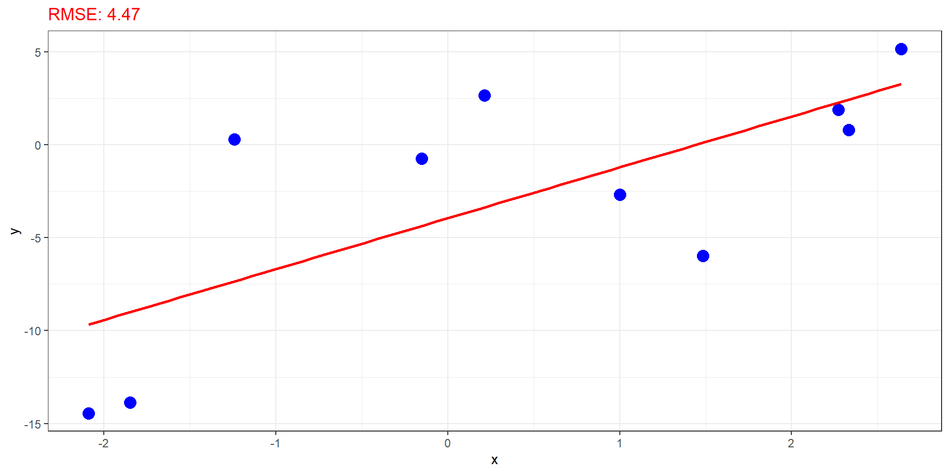
mod1 <-lm(y ~ x, data = d[d$sample, ])rmse1 <-sqrt(mean(resid(mod1)^2))ggplot(aes(x = x, y = y), data = d[d$sample, ]) +geom_point(color ="blue", size =4) +geom_smooth(method ="lm", color ="red", se =FALSE, formula = y ~ x) +labs(title =paste("RMSE:", round(rmse1, 2))) +theme_bw() +theme(plot.title =element_text(color ="red"))
Code
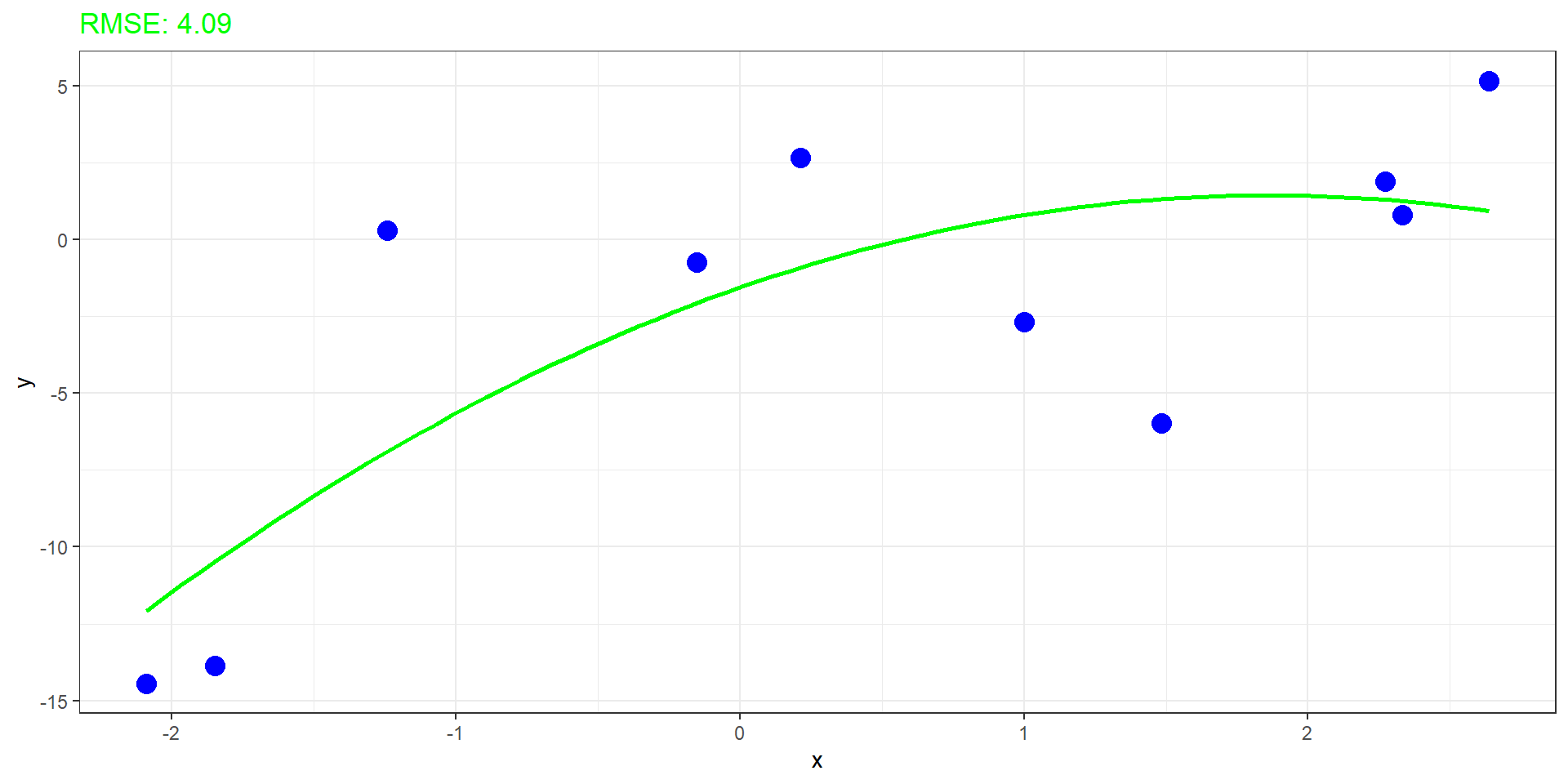
mod2 <-lm(y ~poly(x, 2), data = d[d$sample, ])rmse2 <-sqrt(mean(resid(mod2)^2))ggplot(aes(x = x, y = y), data = d[d$sample, ]) +geom_point(color ="blue", size =4) +geom_smooth(method ="lm", color ="green", se =FALSE, formula = y ~poly(x, 2)) +labs(title =paste("RMSE:", round(rmse2, 2))) +theme_bw() +theme(plot.title =element_text(color ="green"))
Code
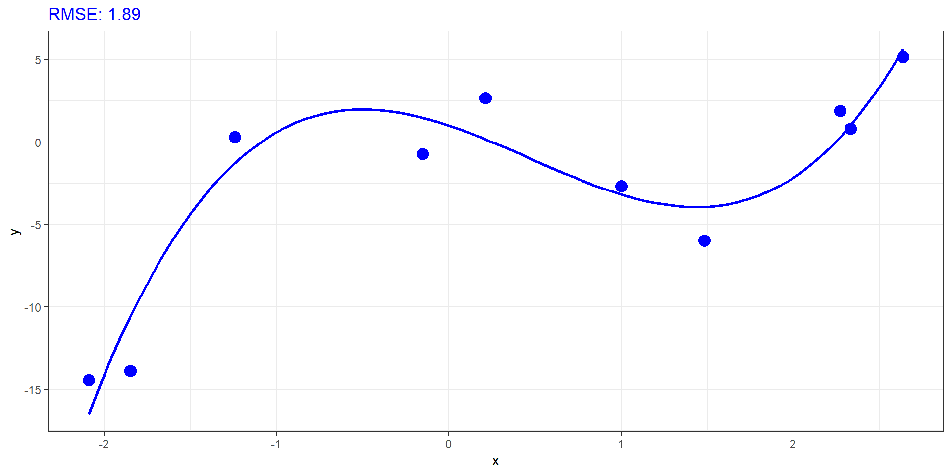
mod3 <-lm(y ~poly(x, 3), data = d[d$sample, ])rmse3 <-sqrt(mean(resid(mod3)^2))ggplot(aes(x = x, y = y), data = d[d$sample, ]) +geom_point(color ="blue", size =4) +geom_smooth(method ="lm", color ="blue", se =FALSE, formula = y ~poly(x, 3)) +labs(title =paste("RMSE:", round(rmse3, 2))) +theme_bw() +theme(plot.title =element_text(color ="blue"))
Code
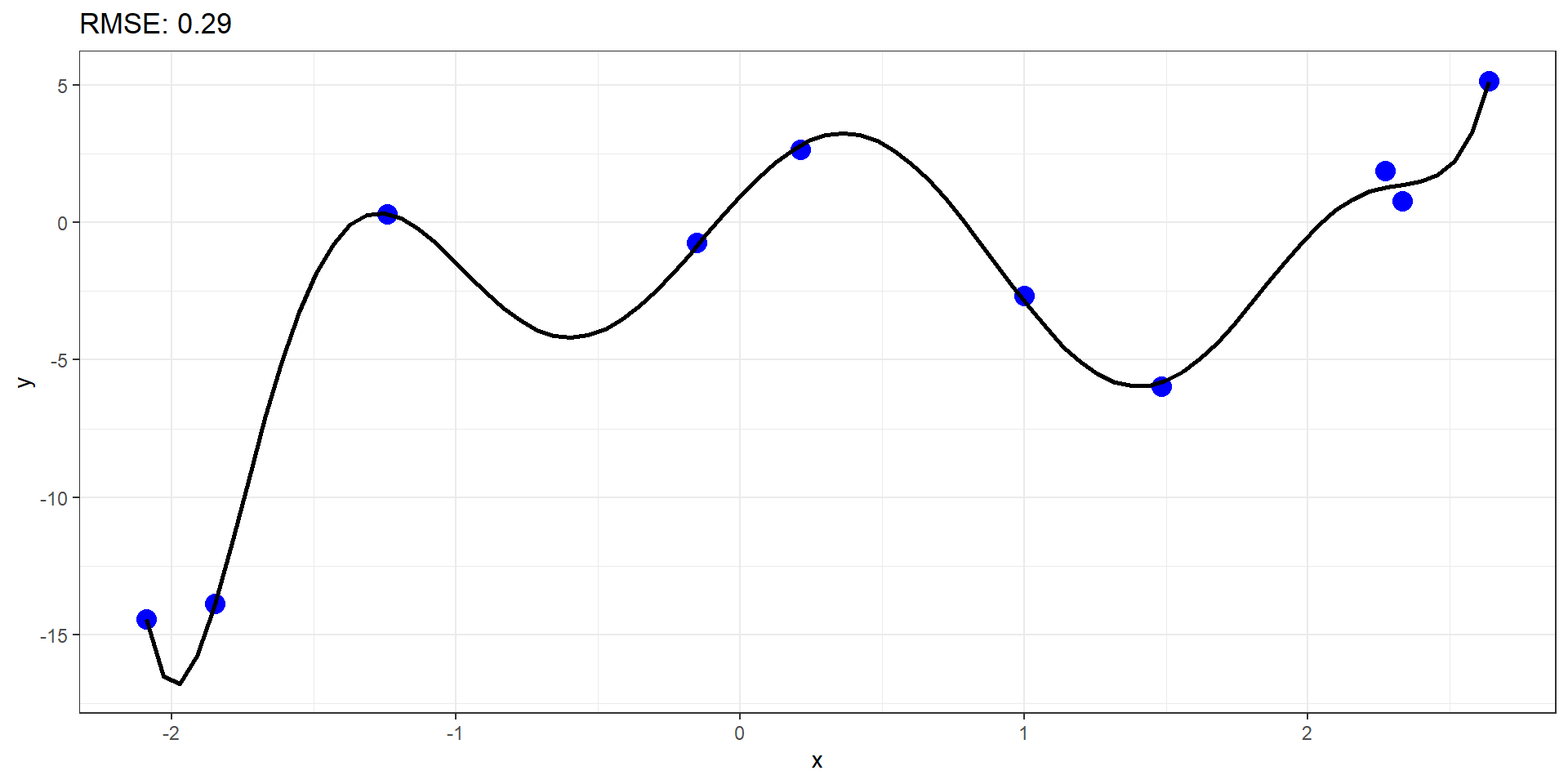
mod8 <-lm(y ~poly(x, 8), data = d[d$sample, ])rmse8 <-sqrt(mean(resid(mod8)^2))ggplot(aes(x = x, y = y), data = d[d$sample, ]) +geom_point(color ="blue", size =4) +geom_smooth(method ="lm", color ="black", se =FALSE, formula = y ~poly(x, 8)) +labs(title =paste("RMSE:", round(rmse8, 2))) +theme_bw() +theme(plot.title =element_text(color ="black"))
Überblick Modelle
Code
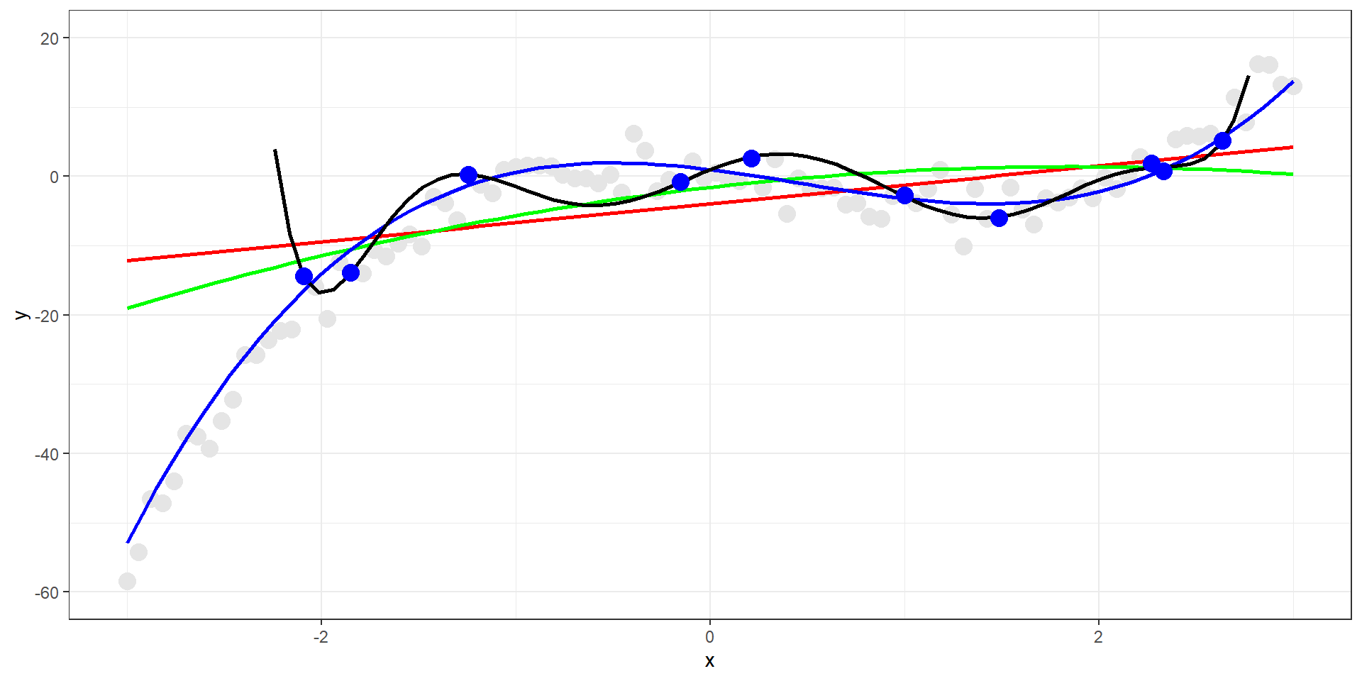
ggplot(aes(x = x, y = y), data = d[d$sample, ]) +geom_point(data = d[!d$sample, ], color ="grey90", size =4) +geom_smooth(method ="lm", color ="red", se =FALSE, formula = y ~ x, fullrange =TRUE) +geom_smooth(method ="lm", color ="green", se =FALSE, formula = y ~poly(x, 2), fullrange =TRUE) +geom_smooth(method ="lm", color ="blue", se =FALSE, formula = y ~poly(x, 3), fullrange =TRUE) +geom_smooth(method ="lm", color ="black", se =FALSE, formula = y ~poly(x, 8), fullrange =TRUE) +geom_point(color ="blue", size =4) +scale_y_continuous(limits =c(-60, 20)) +theme_bw() +theme(plot.title =element_text(color ="black"))
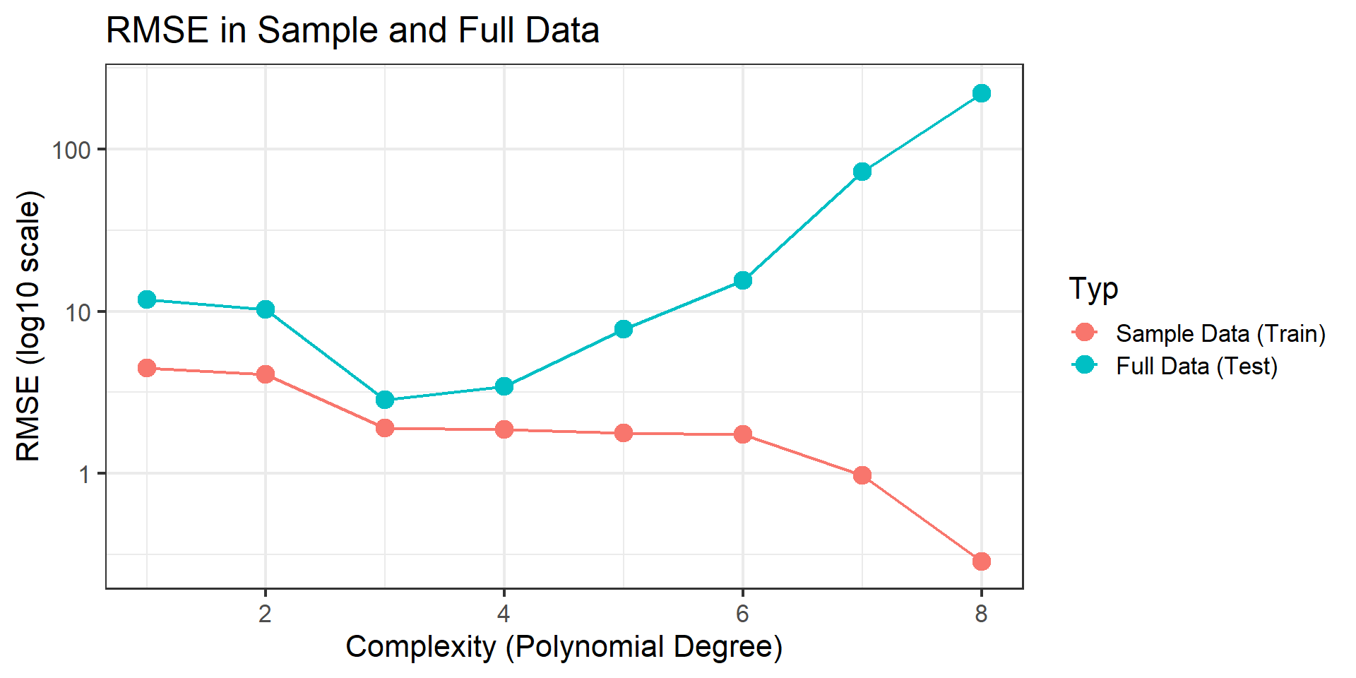
RMSE in Sample vs. Full Data
Code
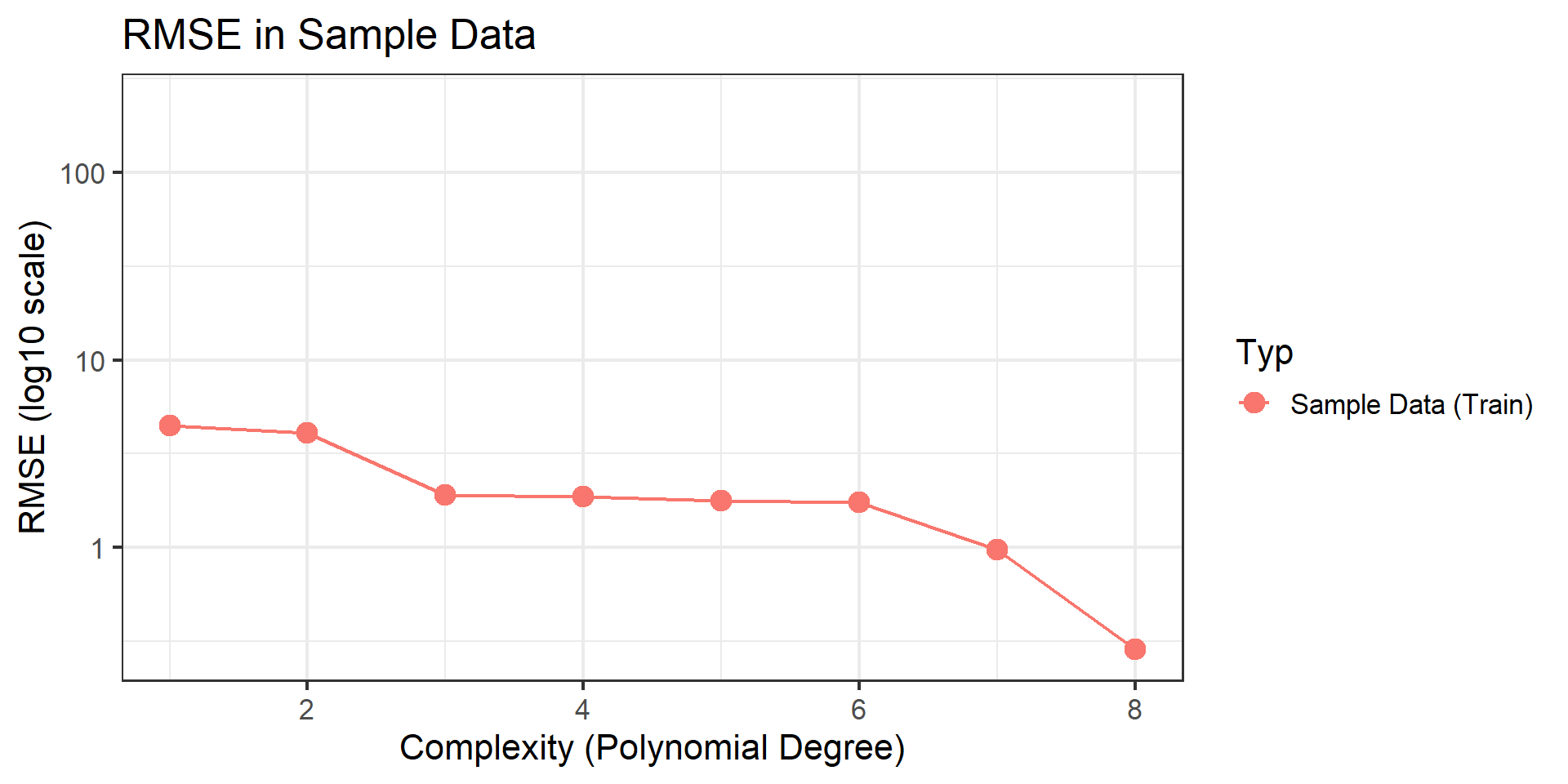
# Funktion um RSME in sample und full data zu berechnen in Abhängigkeit von Polynomgradcalc_rmse <-function(order) { mod_sample <-lm(y ~poly(x, order), data = d[d$sample, ]) rmse_sample <-sqrt(mean(resid(mod_sample)^2)) mod_full_resid <-predict(mod_sample, newdata = d) - d$y rmse_full <-sqrt(mean(mod_full_resid^2))data.frame(order = order,rmse_sample = rmse_sample, rmse_full = rmse_full)}rmse <-lapply(1:8, calc_rmse) |> purrr::list_rbind()rmse <- tidyr::pivot_longer(rmse, cols =c("rmse_sample", "rmse_full"), names_to ="type", values_to ="rmse")rmse$type <-factor(rmse$type, levels =c("rmse_sample", "rmse_full"), labels =c("Sample Data (Train)", "Full Data (Test)"))p1 <-ggplot(rmse[rmse$type =="Sample Data (Train)",], aes(x = order, y = rmse, color = type)) +geom_point(size =4) +geom_line() +scale_y_log10(limits =c(0.27, 240)) +labs(title ="RMSE in Sample Data", x ="Complexity (Polynomial Degree)", y ="RMSE (log10 scale)", color ="Typ") +theme_bw(base_size =16) +theme()p2 <-ggplot(rmse, aes(x = order, y = rmse, color = type)) +geom_point(size =4) +geom_line() +scale_y_log10(limits =c(0.27, 240)) +labs(title ="RMSE in Sample and Full Data", x ="Complexity (Polynomial Degree)", y ="RMSE (log10 scale)", color ="Typ") +theme_bw(base_size =16) +theme()
Bias & Variance
Bias
Wie nah liegt mein Modell an den Daten
Variance
Wie wenig ändert sich mein Modell bei anderer Stichprobe
Generelle Regeln:
weniger komplexe Modelle: low variance, high bias (underfitting)
komplexere Modelle: high variance, low bias (overfitting)
Für gute Vorhersagen brauchen wir das Optimum zwischen bias und variance
Train/Test Split
Train vs. Test Data
In meiner Sample ist mein Modell immer besser als in neuen Daten
Uns interessiert aber eigentlich nur die Performance in neuen Daten
Zwei Möglichkeiten:
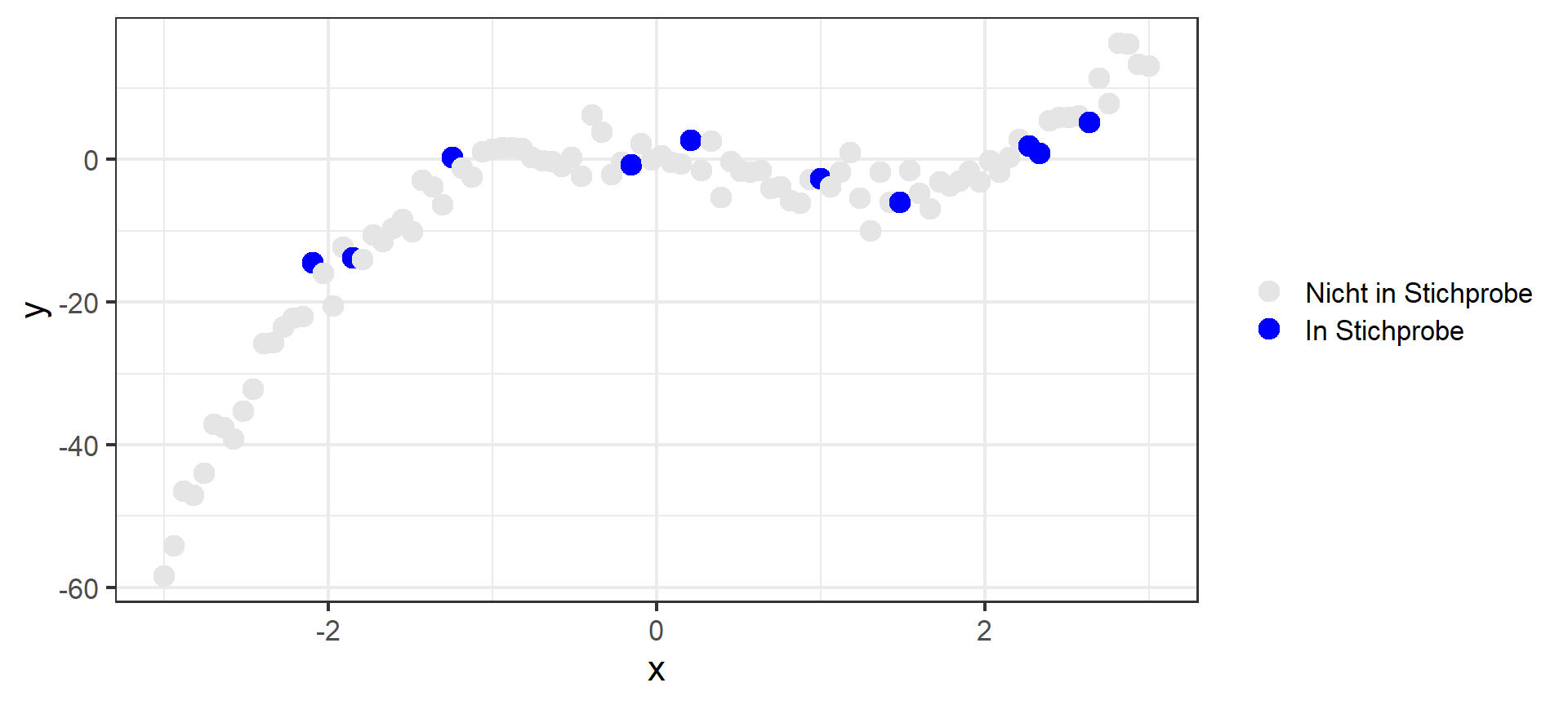
Model in alten Daten fitten, dann neue Daten sammeln und testen
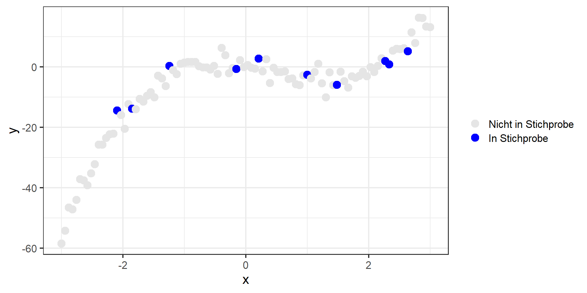
ggplot(d, aes(x = x, y = y, color = sample)) +geom_point(size =4) +scale_color_manual(values =c("grey90", "blue"), labels =c("Nicht in Stichprobe", "In Stichprobe"), name =NULL) +theme_bw(base_size =16)
Wie finde ich den besten Wert für meinen Hyperparameter ohne Testset zu benutzen?
Cross-Validation
Ich mache verschiedene Splits, fitte jeweils neu, evaluiere jeweils neu, dann mitteln
Beispiel: 5-fold CV: Ich teile meinen Train-Datensatz in 5 Teile (4 Train, 1 Validation), mache das 5 mal, sodass jedes Teil einmal Validation ist
Cross-Validation in R
set.seed(123)mod2 <-lm(y ~poly(x, 2), data = dtrain)res <- cv::cv(mod2, k =5)as.data.frame(res)
  fold      mse adjusted.mse full.mse coef.Intercept coef.poly(x, 2)1
1    0 35.06370       32.774   16.719       -2.68995           14.484
2    1  0.29632           NA       NA       -2.71838           14.391
3    2 25.57694           NA       NA       -2.66467           12.455
4    3 39.83809           NA       NA       -3.50123           16.968
5    4 27.50860           NA       NA       -3.49876           11.531
6    5 82.09853           NA       NA       -0.91005           17.267
  coef.poly(x, 2)2
1          -5.7190
2          -5.7533
3          -2.2789
4          -4.6987
5          -8.4606
6         -10.4657
Cross-Validation für Hyperparamter-Tuning
Code
# Funktion um RMSE für gegebenen Polynomgrad zu berechnencalc_cv_rmse <-function(order, data) {set.seed(123)lm(y ~poly(x, degree = order), data = data) mod <-lm(data$y ~poly(data$x, degree = order)) res <- cv::cv(mod, k =5)data.frame(order = order, rmse_cv =as.data.frame(res)$mse[1])}# Funktion auf Polynomgrade 1 bis 6 anwenden und Ergebnisse in Tabelle anzeigenlapply(1:6, calc_cv_rmse, data = dtrain) |> purrr::list_rbind() |> knitr::kable(col.names =c("Polynomgrad", "CV RMSE"))
Polynomgrad
CV RMSE
1
25.03841
2
35.06370
3
12.86487
4
20.97448
5
228.74941
6
550.08656
Workflow
Train/Test Split, Testset beiseitelegen
In Trainset: bestes Modell auswählen (z.B. durch CV)