               name position          school       college height weight sprint
1          BJ Adams       CB Central Florida College Stats 187.96   82.6   4.53
2 Tommy Akingbesote       DT        Maryland College Stats 193.04  138.8   5.09
3  Darius Alexander       DT          Toledo College Stats 193.04  138.3   4.95
4      Zy Alexander       CB             LSU College Stats 185.42   84.8   4.56
5     LeQuint Allen       RB        Syracuse College Stats 182.88   92.5     NA
6         Trey Amos       CB     Mississippi College Stats 185.42   88.5   4.43
  jump_vertical bench jump_broad cone shuttle drafted
1         82.55    NA     297.18   NA      NA   FALSE
2         71.12    NA     261.62   NA      NA    TRUE
3         80.01    28     281.94  7.6    4.79    TRUE
4         80.01    NA     294.64   NA      NA   FALSE
5         88.90    NA     304.80   NA      NA    TRUE
6 82.55 13 320.04 NA NA TRUELogistische Regression
Problemstellung
Beispiel: NFL Combine
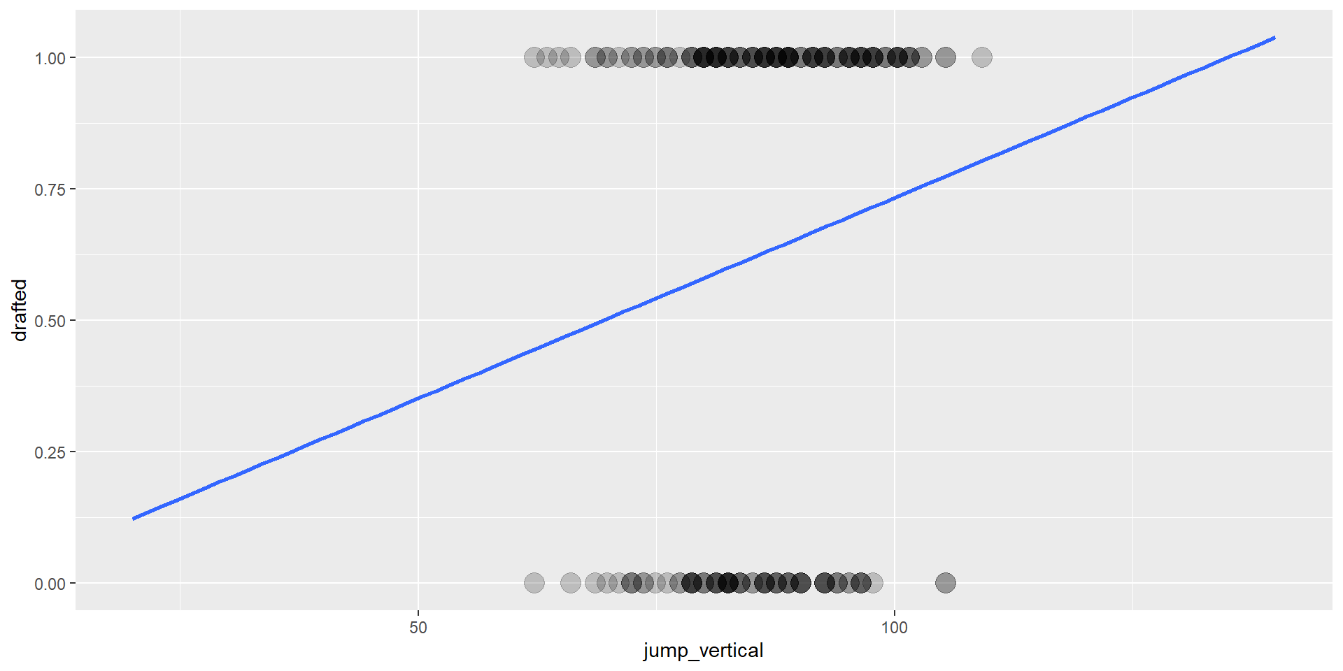
Problem: binäres Outcome
- wir möchten eine Wahrscheinlichkeit vorhersagen
- Wahrscheinlichkeiten sind zwischen 0 und 1
- lineare Modelle können Werte außerhalb dieses Bereichs vorhersagen
Grundlagen Logistische Regression
Lösung Teil 1: Odds
- Odds = Wahrscheinlichkeit ja / Wahrscheinlichkeit nein
- z.B. Odds von 1:1 (1) -> 50% Wahrscheinlichkeit
- z.B. Odds von 2:1 (2) -> 66.7% Wahrscheinlichkeit
- z.B. Odds von 1:2 (0.5) -> 33.3% Wahrscheinlichkeit
- Wertebereich Odds: 0 bis +unendlich
- allgemeine Formel: \(odds = \frac{p}{1-p}\)
Lösung Teil 2: Logit
- Logit = log(Odds)
- z.B. Logit von 1:1 (1) -> 0
- z.B. Logit von 2:1 (2) -> 0.693
- z.B. Logit von 1:2 (0.5) -> -0.693
- Wertebereich Logit: -unendlich bis +unendlich
- allgemeine Formel: \(\text{Logit} = \log\left(\frac{p}{1-p}\right)\)
Übersicht
| P | Odds | Logit |
|---|---|---|
| 0.5 | 1 | 0 |
| 0 | 0 | \(-\infty\) |
| 1 | \(\infty\) | \(\infty\) |
Formel
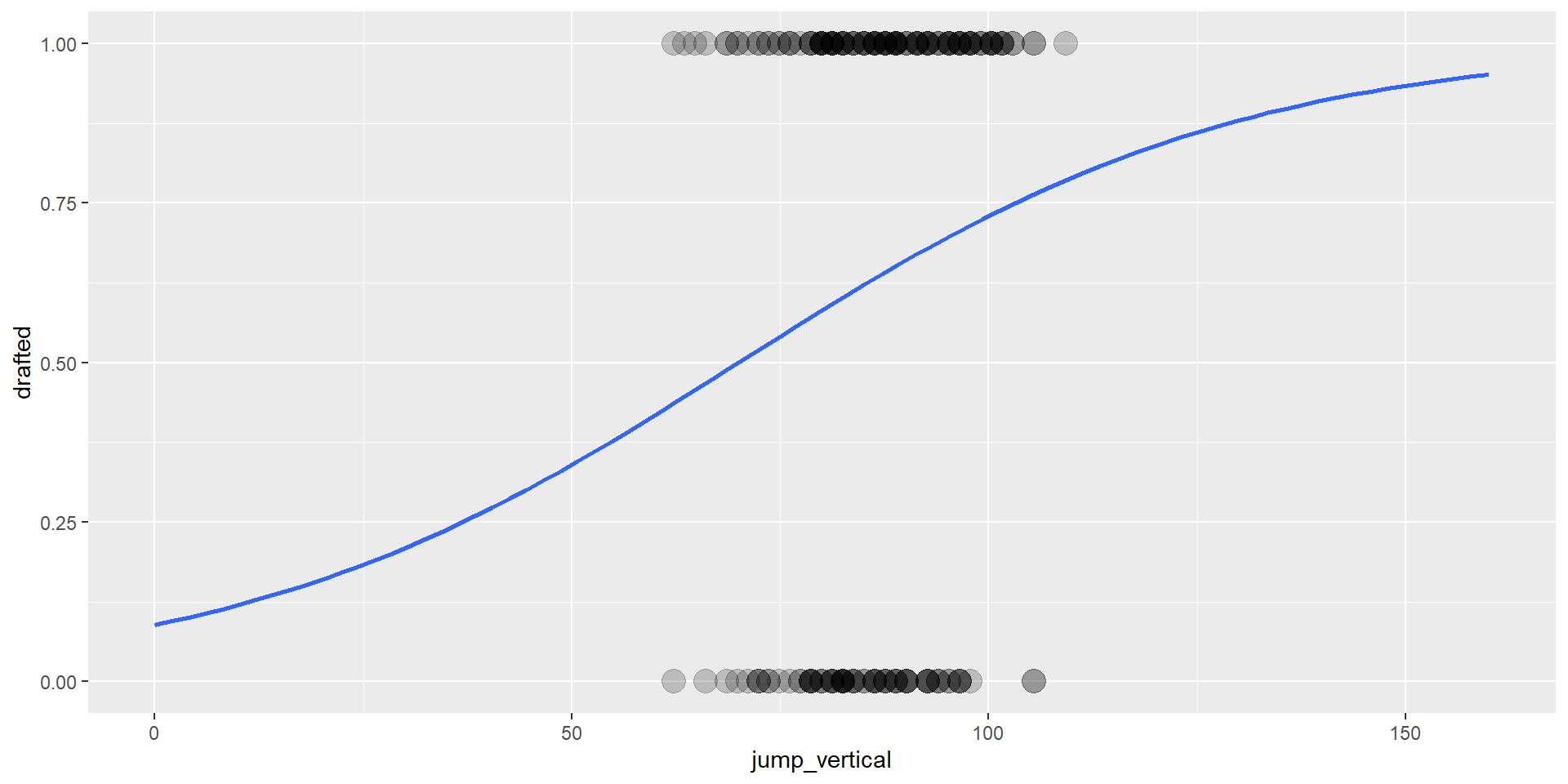
\[\text{logit}(p) = \beta_0 + \beta_1 x\]
Interaktives Beispiel
viewof b = Inputs.range([-5, 5], {value: 0, step: 0.1, label: "Intercept"})
viewof m = Inputs.range([-3, 3], {value: 1, step: 0.1, label: "Slope"})

function lineData(b, m){
  const pts = [];
  for(let x = -10; x <= 10; x += 0.5) pts.push({x, y: b + m * x});
  return pts;
}

function probData(b, m){
  const pts = [];
  for(let x = -10; x <= 10; x += 0.5){
    const lin = b + m * x;
    const p = 1 / (1 + Math.exp(-lin));
    pts.push({x, p});
  }
  return pts;
}
{
const width = 680;
const height = 220;
const container = document.createElement("div");
container.style.display = "flex";
container.style.flexDirection = "column";
container.style.gap = "12px";
const logitPlot = Plot.plot({
width, height,
x: {domain: [-10, 10], label: "x"},
y: {domain: [-10, 10], label: "Log-Odds"},
marks: [
Plot.line(lineData(b, m), {x: "x", y: "y", stroke: "steelblue", strokeWidth: 3}),
Plot.ruleY([0], {stroke: "#333"}),
Plot.ruleX([0], {stroke: "#333"})
]
});
const probPlot = Plot.plot({
width, height,
x: {domain: [-10, 10], label: "x"},
y: {domain: [0, 1], label: "Probability"},
marks: [
Plot.line(probData(b, m), {x: "x", y: "p", stroke: "tomato", strokeWidth: 3}),
Plot.ruleY([0.5], {stroke: "#333", strokeDasharray: "4,4"}),
Plot.ruleX([0], {stroke: "#333"})
]
});
container.appendChild(logitPlot);
container.appendChild(probPlot);
return container;
}Berechnen & Interpretieren
Logistische Regression fitten
- least squares passt nicht so gut, daher wird maximum likelihood estimation verwendet
# A tibble: 2 × 7
  term          estimate std.error statistic p.value conf.low conf.high
  <chr>            <dbl>     <dbl>     <dbl>   <dbl>    <dbl>     <dbl>
1 (Intercept)    -2.32      1.35       -1.72  0.0853 -5.02       0.300
2 jump_vertical   0.0332    0.0157      2.12  0.0342  0.00286    0.0645
Vorsicht: Die Skala sind log-Odds
Wenn jump = 0, log-Odds gedraftet zu werden -> -2.32
pro +1cm jump, log-Odds gedraftet zu werden: +0.03
Umrechnung in Odds
- Exponent nehmen \(e^x\) (Gegenteil von Log)
glm(drafted ~ jump_vertical, data = nfl2025, family = binomial) |>
  broom::tidy(exponentiate = TRUE, conf.int = TRUE)
# A tibble: 2 × 7
term estimate std.error statistic p.value conf.low conf.high
<chr> <dbl> <dbl> <dbl> <dbl> <dbl> <dbl>
1 (Intercept) 0.0979 1.35 -1.72 0.0853 0.00662 1.35
2 jump_vertical 1.03 0.0157 2.12 0.0342 1.00 1.07Vorsicht: Die Skala sind Odds
Wenn jump = 0, Odds gedraftet zu werden -> 0.10 (~ 9% Wahrscheinlichkeit)
pro +1cm jump, Odds gedraftet zu werden: mal 1.03
Vorhersage
Log-Odds
new_data <- data.frame(jump_vertical = c(50, 60, 70, 80, 90, 100))
insight::get_predicted(nfl_mod, data = new_data, predict = "link", ci = 0.95) |>
  as.data.frame()
Predicted SE CI_low CI_high
1 -0.6642623655 0.5776785 -1.796491385 0.4679667
2 -0.3324465703 0.4278745 -1.171065220 0.5061721
3 -0.0006307751 0.2855152 -0.560230313 0.5589688
4 0.3311850201 0.1704096 -0.002811632 0.6651817
5 0.6630008153 0.1601189 0.349173474 0.9768282
6 0.9948166105 0.2670484 0.471411267 1.5182220Vorhersage Wahrscheinlichkeiten
new_data <- data.frame(jump_vertical = c(50, 60, 70, 80, 90, 100))
insight::get_predicted(nfl_mod, data = new_data, predict = "expectation", ci = 0.95) |>
  as.data.frame()
Predicted SE CI_low CI_high
1 0.3397828 0.12959087 0.1422787 0.6149024
2 0.4176455 0.10406667 0.2366625 0.6239087
3 0.4998423 0.07137880 0.3634942 0.6362139
4 0.5820477 0.04145523 0.4992971 0.6604234
5 0.6599342 0.03593406 0.5864171 0.7264784
6 0.7300382 0.05263055 0.6157177 0.8202765Vorhersage Klassifikation
benötigt Vorhersageregel, z.B. \(p < 0.5 \rightarrow 0, p \ge 0.5 \rightarrow 1\)
new_data <- data.frame(jump_vertical = c(50, 60, 70, 80, 90, 100))
insight::get_predicted(nfl_mod, data = new_data, predict = "classification")
Predicted values:
[1] 0 0 0 1 1 1
NOTE: Confidence intervals, if available, are stored as attributes and can be accessed using `as.data.frame()` on this output.Modellqualität (Abgleich Vorhersage vs. Realität)
Konfusionsmatrix
| Actual Negative | Actual Positive | |
|---|---|---|
| Predicted Negative | True Negative | False Negative |
| Predicted Positive | False Positive | True Positive |
Accuracy: \(\frac{TP + TN}{total}\)
Sensitivity: \(\frac{TP}{TP + FN}\)
Specificity: \(\frac{TN}{TN + FP}\)
Konfusionsmatrix in R
Confusion Matrix and Statistics

          Reference
Prediction   0   1
         0   4   8
         1  73 123

               Accuracy : 0.6106
                 95% CI : (0.5407, 0.6772)
    No Information Rate : 0.6298
    P-Value [Acc > NIR] : 0.742

                  Kappa : -0.011

 Mcnemar's Test P-Value : 1.151e-12

            Sensitivity : 0.05195
            Specificity : 0.93893
         Pos Pred Value : 0.33333
         Neg Pred Value : 0.62755
             Prevalence : 0.37019
         Detection Rate : 0.01923
   Detection Prevalence : 0.05769
      Balanced Accuracy : 0.49544

       'Positive' Class : 0
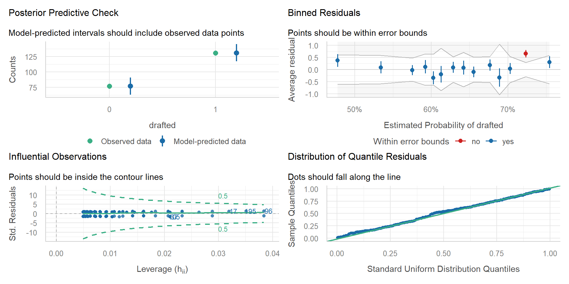
Voraussetzungen
Beispiel
Datensatz
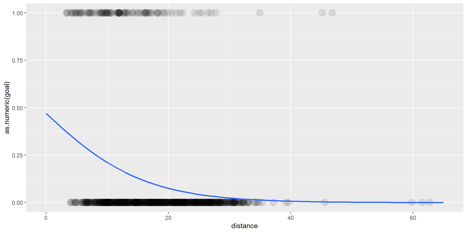
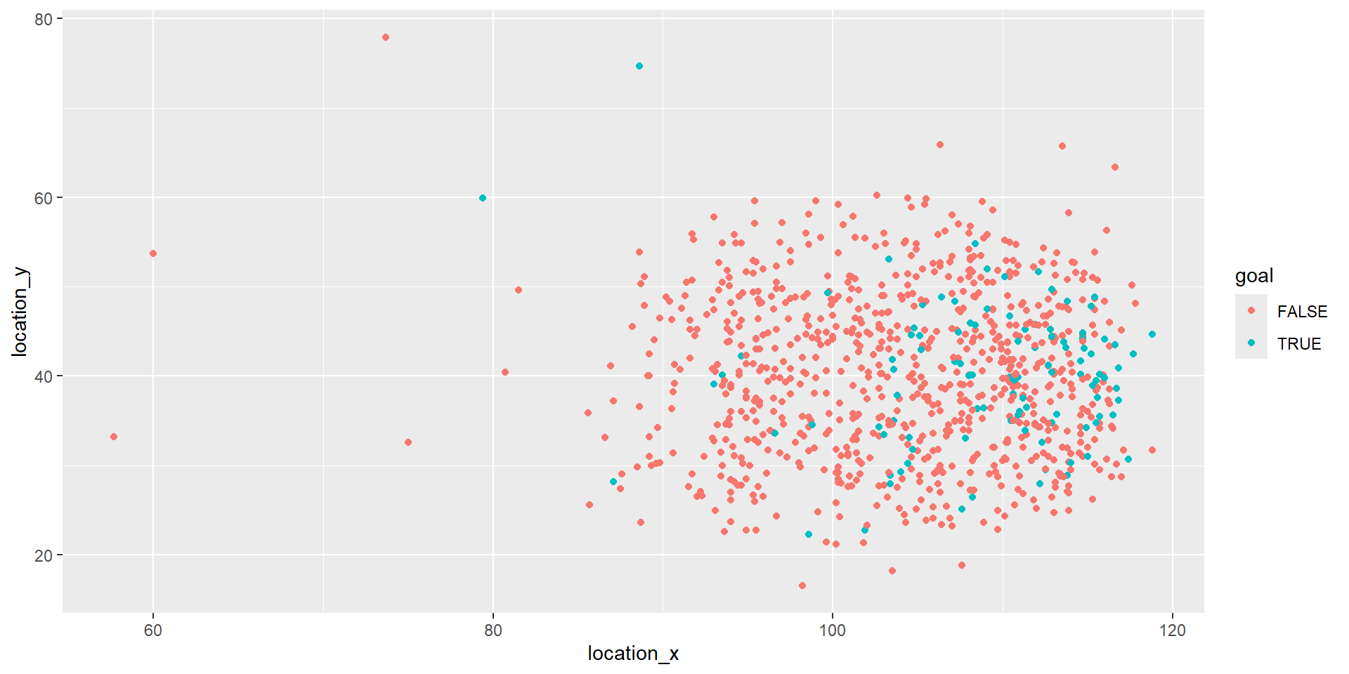
Alle Schüsse aus 34 Bundesliga-Spielen der Saison 2023/2024.
                                    id    timestamp        team.name
1 c577e730-b9f5-44f2-9257-9e7730c23d7b 00:06:48.773    Werder Bremen
2 bbc2c68d-c096-483d-abf4-32c0175a0f55 00:07:40.953 Bayer Leverkusen
  shot.technique.name shot.body_part.name shot.type.name shot.outcome.name
1              Normal          Right Foot      Open Play           Blocked
2              Normal           Left Foot      Open Play             Saved
  location_x location_y  goal  distance
1      100.4       35.1 FALSE 20.203218
2 114.6 33.5 FALSE 8.450444Datensatz
Modell
shots_mod <- glm(goal ~ distance, data = shots, family = binomial)
broom::tidy(shots_mod, exponentiate = TRUE, conf.int = TRUE)
# A tibble: 2 × 7
term estimate std.error statistic p.value conf.low conf.high
<chr> <dbl> <dbl> <dbl> <dbl> <dbl> <dbl>
1 (Intercept) 0.886 0.257 -0.471 6.38e- 1 0.534 1.47
2 distance 0.888 0.0172 -6.94 3.81e-12 0.857 0.917Vorhersagequalität
shots$pred <- insight::get_predicted(shots_mod, predict = "classification")
caret::confusionMatrix(
  as.factor(shots$pred),
  as.factor(shots$goal)
)
Confusion Matrix and Statistics
Reference
Prediction FALSE TRUE
FALSE 806 110
TRUE 0 0
Accuracy : 0.8799
95% CI : (0.8571, 0.9003)
No Information Rate : 0.8799
P-Value [Acc > NIR] : 0.5254
Kappa : 0
Mcnemar's Test P-Value : <2e-16
Sensitivity : 1.0000
Specificity : 0.0000
Pos Pred Value : 0.8799
Neg Pred Value : NaN
Prevalence : 0.8799
Detection Rate : 0.8799
Detection Prevalence : 1.0000
Balanced Accuracy : 0.5000
'Positive' Class : FALSE
Visualisierung