Lineares Modell - Erweiterungen

Wiederholung

Categorical Predictors

Diskrete Variablen

library(sportsdata)
library(ggplot2)

ggplot(olympics, aes(x = sex, y = height)) +
    geom_point(alpha = 0.01)

Diskrete Variablen als Prädiktoren

\[height = \beta_0 + \beta_1 sex \]

• \(sex = 0\) wenn “female”
• \(sex = 1\) wenn “male”
• \(\beta_0\): Mittelwert nur female (y-Achsenabschnitt)
• \(\beta_1\): Unterschied Mittelwert male zu Mittelwert female (Steigung)

Ergebnisse

• Modellevaluation
• Visualisierung

sex_mod <- lm(height ~ sex, data = olympics)
broom::tidy(sex_mod, conf.int = TRUE)

# A tibble: 2 × 7
  term        estimate std.error statistic p.value conf.low conf.high
  <chr>          <dbl>     <dbl>     <dbl>   <dbl>    <dbl>     <dbl>
1 (Intercept)    168.     0.0354     4747.       0    168.      168. 
2 sexM            11.0    0.0429      257.       0     10.9      11.1

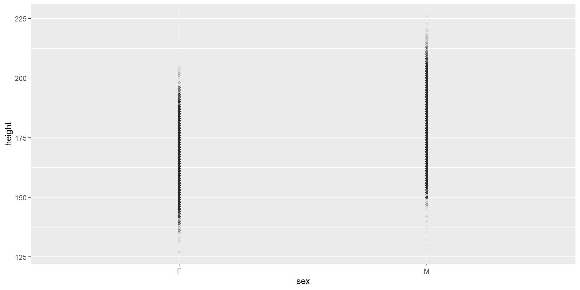
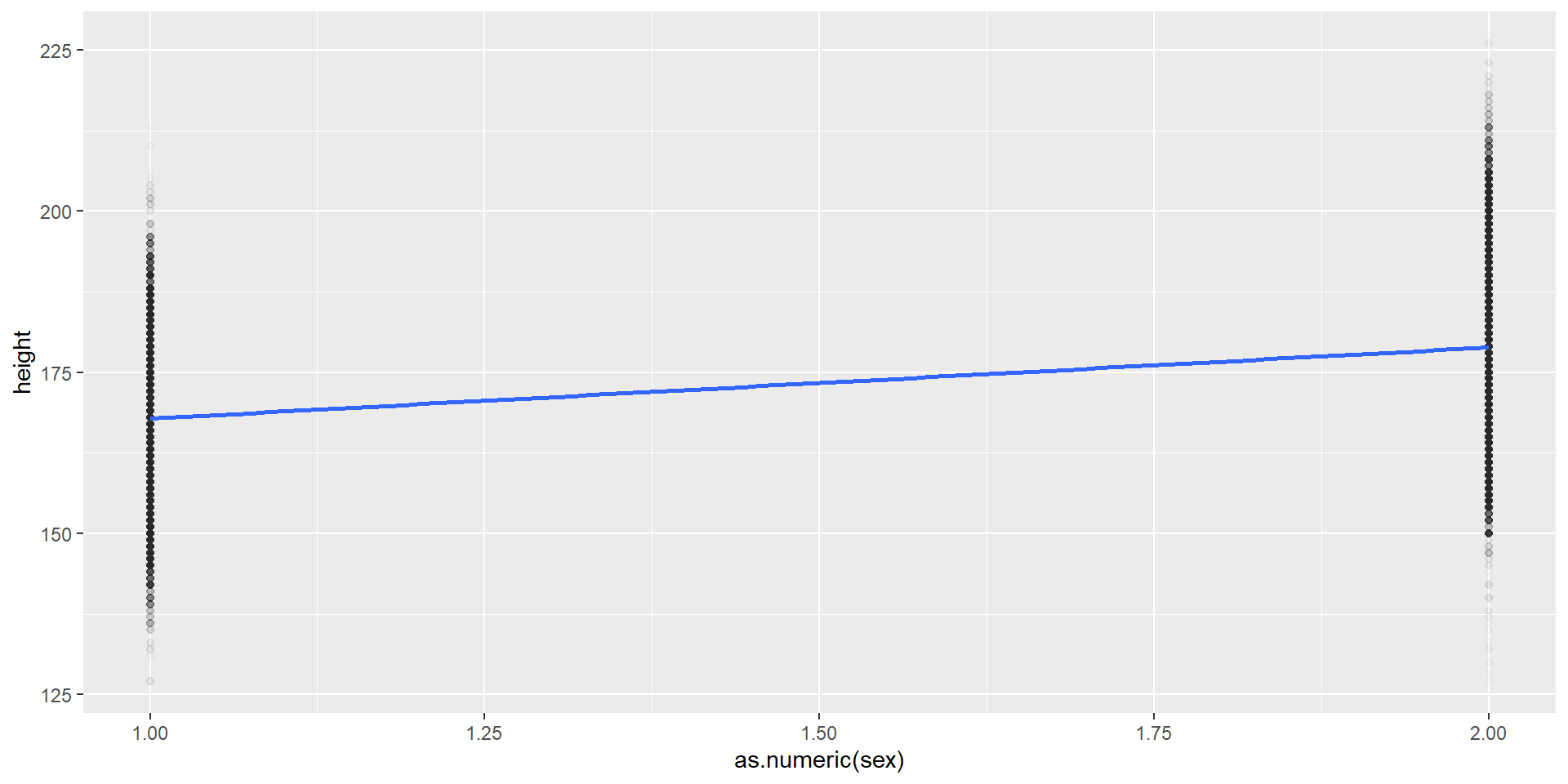
# bei nur diskreten Prädiktoren funktioniert geom_smooth(method = "lm") nicht, daher konvertieren wir zu numerisch
ggplot(olympics, aes(x = as.numeric(sex), y = height)) +
    geom_point(alpha = 0.01) +
    geom_smooth(method = "lm", se = FALSE)

Mehr als zwei Kategorien

• Daten
• Visualisierung

table(olympics$medal,useNA = "ifany")

Bronze   Gold Silver   <NA> 
 13295  13372  13116 231333 

med <- olympics[!is.na(olympics$medal),]
nrow(med)

[1] 39783

ggplot(med, aes(x = medal, y = height)) +
    geom_point(alpha = 0.01)

Dummy-Coding

\[height = \beta_0 + \beta_1 medal \]

\[\Rightarrow height = \beta_0 + \beta_1 medal_1 + \beta_2 medal_2 \]

	medal1	medal2
bronze	0	0
silver	0	1
gold	1	0

Ergebnisse

med_mod <- lm(height ~ medal, data = med)
broom::tidy(med_mod, conf.int = TRUE)

# A tibble: 3 × 7
  term        estimate std.error statistic   p.value conf.low conf.high
  <chr>          <dbl>     <dbl>     <dbl>     <dbl>    <dbl>     <dbl>
1 (Intercept)  177.        0.107   1657.   0          177.      178.   
2 medalGold      0.600     0.151      3.98 0.0000680    0.305     0.895
3 medalSilver    0.160     0.152      1.05 0.293       -0.138     0.458

broom::glance(med_mod)

# A tibble: 1 × 12
  r.squared adj.r.squared sigma statistic  p.value    df   logLik     AIC    BIC
      <dbl>         <dbl> <dbl>     <dbl>    <dbl> <dbl>    <dbl>   <dbl>  <dbl>
1  0.000548      0.000484  10.9      8.52 0.000200     2 -118286. 236580. 2.37e5
# ℹ 3 more variables: deviance <dbl>, df.residual <int>, nobs <int>

Multiple Predictors

Modell: Multiple Regression

\[weight = \beta_0 + \beta_1 sex + \beta_2 height \]

• \(\beta_0\): Gewicht wenn sex = 0 (female) und height = 0
• \(\beta_1\): Unterschied Gewicht wenn sex = 1 (male), unabhängig von Größe
• \(\beta_2\): Veränderung Gewicht pro cm Körpergröße, unabhängig vom Geschlecht

Ergebnisse

multi_mod <- lm(weight ~ sex + height, data = olympics)

• Parameter
• Visualisierung

broom::tidy(multi_mod, conf.int = TRUE)

# A tibble: 3 × 7
  term        estimate std.error statistic p.value conf.low conf.high
  <chr>          <dbl>     <dbl>     <dbl>   <dbl>    <dbl>     <dbl>
1 (Intercept) -104.      0.341       -304.       0 -104.     -103.   
2 sexM           4.94    0.0455       108.       0    4.85      5.03 
3 height         0.975   0.00202      483.       0    0.971     0.979

library(visreg)

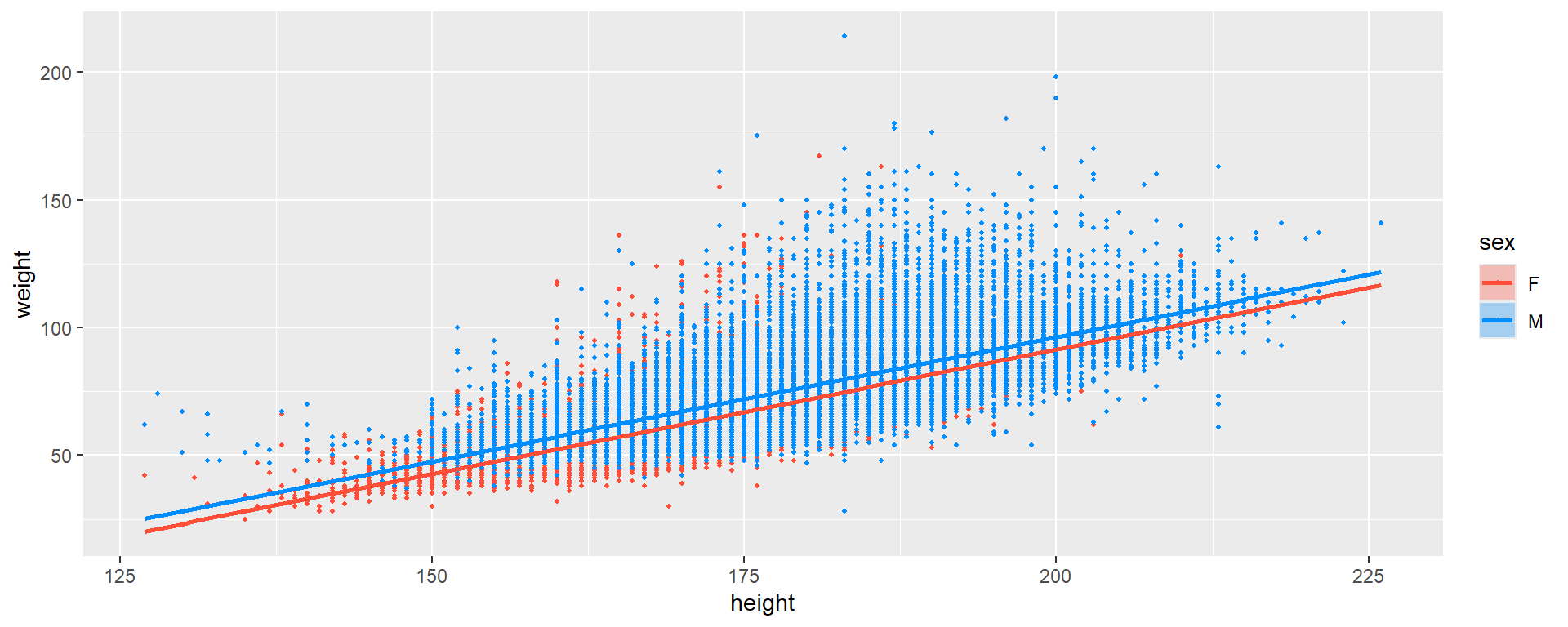
# geom_smooth(method = "lm") malt Linien die nicht zwingend parallel sind, daher nutzen wir visreg
visreg(multi_mod, xvar = "height", by = "sex", overlay = TRUE, gg = TRUE)

Modellvergleich

mod_sex <- lm(weight ~ sex, data = olympics)
mod_height <- lm(weight ~ height, data = olympics)

g1 <- broom::glance(mod_sex)
g2 <- broom::glance(mod_height)
g3 <- broom::glance(multi_mod)

rbind(g1, g2, g3)

# A tibble: 3 × 12
  r.squared adj.r.squared sigma statistic p.value    df   logLik      AIC    BIC
      <dbl>         <dbl> <dbl>     <dbl>   <dbl> <dbl>    <dbl>    <dbl>  <dbl>
1     0.262         0.262 12.3     73761.       0     1 -818582. 1637171. 1.64e6
2     0.634         0.634  8.67   358247.       0     1 -740289. 1480585. 1.48e6
3     0.654         0.654  8.43   195183.       0     2 -734571. 1469151. 1.47e6
# ℹ 3 more variables: deviance <dbl>, df.residual <int>, nobs <int>

Mehrere kontinuierliche Prädiktoren

mod_age <- lm(weight ~ height + age, data = olympics)
broom::glance(mod_age)

# A tibble: 1 × 12
  r.squared adj.r.squared sigma statistic p.value    df   logLik      AIC    BIC
      <dbl>         <dbl> <dbl>     <dbl>   <dbl> <dbl>    <dbl>    <dbl>  <dbl>
1     0.645         0.645  8.55   186933.       0     2 -734938. 1469884. 1.47e6
# ℹ 3 more variables: deviance <dbl>, df.residual <int>, nobs <int>

broom::tidy(mod_age, conf.int = TRUE)

# A tibble: 3 × 7
  term        estimate std.error statistic p.value conf.low conf.high
  <chr>          <dbl>     <dbl>     <dbl>   <dbl>    <dbl>     <dbl>
1 (Intercept) -122.      0.316      -387.        0 -123.     -122.   
2 height         1.06    0.00180     590.        0    1.06      1.07 
3 age            0.265   0.00347      76.3       0    0.258     0.272

Visualisierung

a <- 10:70
h <- 120:220
new <- expand.grid(height = h, age = a, KEEP.OUT.ATTRS = FALSE)
new$weight <- predict(mod_age, newdata = new)
r <- reshape2::acast(new, age ~ height, value.var = "weight")
plotly::plot_ly(olympics, x = ~height, y = ~age, z = ~weight, type = "scatter3d", marker = list(size = 2), mode = "markers") |>
    plotly::add_trace(x = h, y = a, z = r, type = "surface")

Voraussetzungen

performance::check_model(mod_age, base_size = 7)