Lineares Modell

Das lineare Modell

Grundlagen

\[y = \beta_0 + \beta_1 x + \epsilon\]

• \(y\): Outcome
• \(x\): Predictor
• \(\beta_0\): y-Achsenabschnitt
• \(\beta_1\): Steigung
• \(\epsilon\): Fehlerterm

Interaktives Beispiel

viewof b = Inputs.range([-5, 5], {value: 2, step: 0.1, label: "Intercept"})
viewof m = Inputs.range([-3, 3], {value: 1, step: 0.1, label: "Slope"})

function lineData(b, m){
  const pts = [];
  for(let x = -10; x <= 10; x += 0.5) pts.push({x, y: b + m * x});
  return pts;
}

Plot.plot({
    width: 600, height: 400,
    x: {domain: [-10, 10]},
    y: {domain: [-10, 10]},
    marks: [
      Plot.line(lineData(b, m), {x: "x", y: "y", stroke: "steelblue", strokeWidth: 3}),
      Plot.ruleY([0], {stroke: "#333"}),
      Plot.ruleX([0], {stroke: "#333"})
    ]
})

Ein lineares Modell fitten

• Residuen: Abweichung der Daten vom Modell
• Root of Mean Squared Error (RSME): “Durchschnittliche” Abweichung
• Ziel: Parameter so wählen, dass RSME minimiert wird

Interaktives Beispiel

import {Inputs} from "@observablehq/inputs"

viewof b2 = Inputs.range([-5, 5], {value: 2, step: 0.1, label: "Intercept"})
viewof m2 = Inputs.range([-3, 3], {value: 1, step: 0.01, label: "Slope"})

// five sample points near y = 2 + 1*x with controlled noise (RMSE ≈ 1.75 at b=2,m=1)
data2 = [
  {x: -4, y: -0.8},
  {x: -2, y: -2.4},
  {x:  0, y:  2.0},
  {x:  2, y:  6.4},
  {x:  4, y:  4.8}
]

function predict2(b, m, x){ return b + m * x }

function residuals2(b, m){
  return data2.map(d => ({x: d.x, y: d.y, yhat: predict2(b, m, d.x), resid: d.y - predict2(b, m, d.x)}));
}

// show RMSE in the sidebar (no imports, no const)
rmse2 = Math.sqrt(residuals2(b2, m2).reduce(function(s,p){return s + p.resid*p.resid}, 0) / residuals2(b2, m2).length)
html`<div style='font-family:sans-serif;margin-top:8px'>RMSE: <strong>${rmse2.toFixed(2)}</strong></div>`

pts2 = residuals2(b2, m2)

linePts2 = [{x: -10, y: predict2(b2, m2, -10)}, {x: 10, y: predict2(b2, m2, 10)}]

// build two-point segments grouped by gid so each draws as a vertical line
segs = pts2.flatMap((p, i) => [{x: p.x, y: p.y, gid: i}, {x: p.x, y: p.yhat, gid: i}])

Plot.plot({
  width: 600, height: 400,
  x: {domain: [-10, 10]},
  y: {domain: [-10, 10]},
  marks: [
    Plot.line(linePts2, {x: "x", y: "y", stroke: "steelblue", strokeWidth: 3}),
    Plot.line(segs, {x: "x", y: "y", z: "gid", stroke: "tomato", strokeWidth: 1.5}),
    Plot.dot(pts2, {x: "x", y: "y", fill: "#000", r: 5}),
    Plot.dot(pts2, {x: "x", y: "yhat", fill: "steelblue", r: 3}),
    Plot.ruleY([0], {stroke: "#333"}),
    Plot.ruleX([0], {stroke: "#333"})
  ]
})

Lineares Modell fitten in R

# Datensatz aus interaktivem Beispiel
df_demo <- data.frame(x = c(-4, -2, 0, 2, 4), y = c(-0.8, -2.4, 2.0, 6.4, 4.8))

# Lineares Modell fitten
# y wird vorhergesagt (~) durch x, unter Nutzung des Datensatzes df_demo
mod <- lm(y ~ x, data = df_demo)
s <- summary(mod)
s$sigma

[1] 2.19089

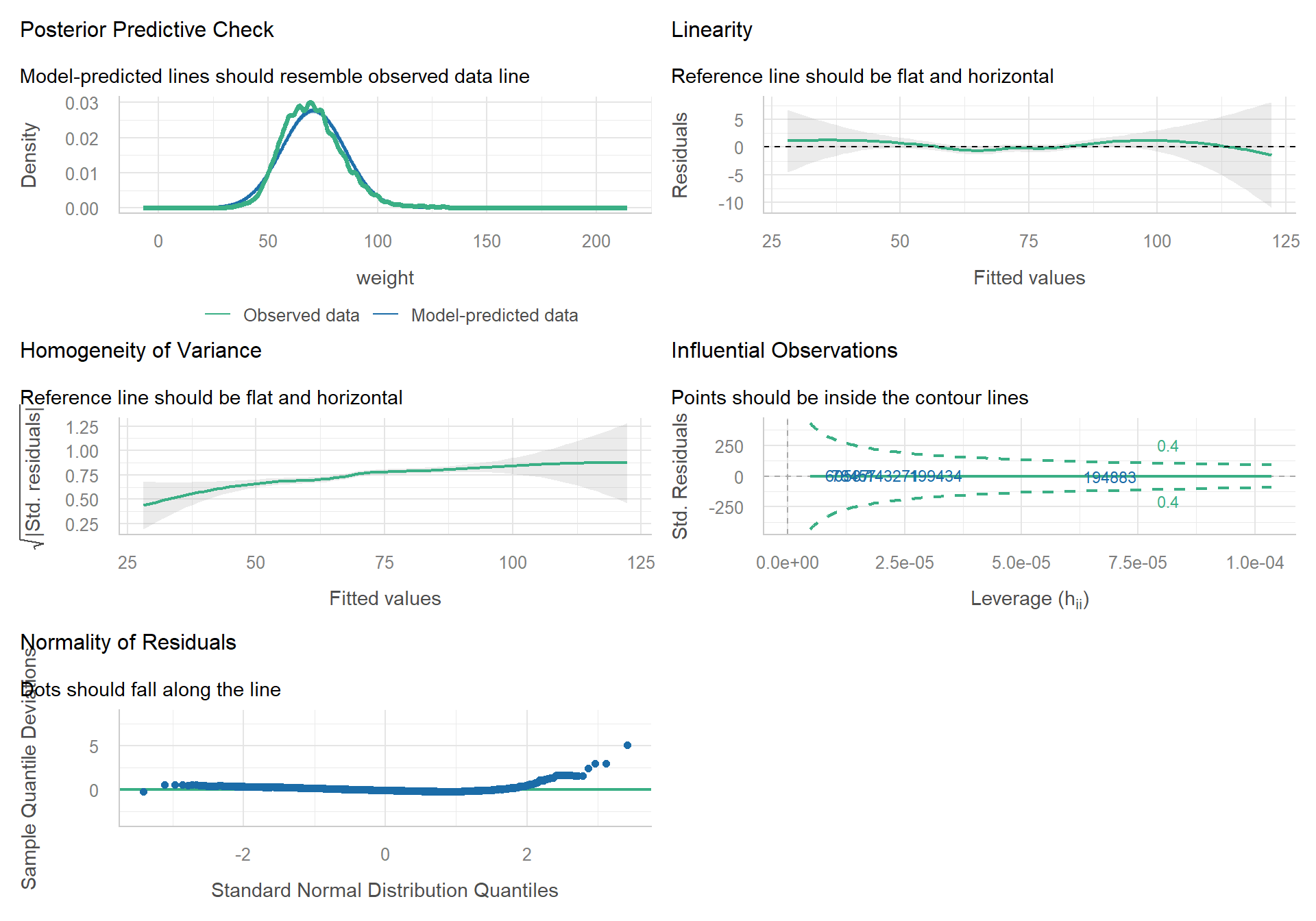
Modellevaluation 1: Gesamtmodell

• Residual Standard Error (RSE): Eine Variante vom RMSE
• R²: Anteil der Streuung, die durch das Modell erklärt wird (100% = alle Punkte liegen auf der Linie)
• F-Statistik & p-Wert: Ist das Modell besser als nur der Mittelwert?

broom::glance(mod)

# A tibble: 1 × 12
  r.squared adj.r.squared sigma statistic p.value    df logLik   AIC   BIC
      <dbl>         <dbl> <dbl>     <dbl>   <dbl> <dbl>  <dbl> <dbl> <dbl>
1     0.735         0.647  2.19      8.33  0.0632     1  -9.74  25.5  24.3
# ℹ 3 more variables: deviance <dbl>, df.residual <int>, nobs <int>

Modellevaluation 2: Parameter

• Standardfehler: Wie sicher ist die Schätzung des Parameters?
• t-Statistik & p-Wert: Leistet der Parameter einen Beitrag zum Modell (Unterscheidet sich der Parameter-Wert von 0)?

broom::tidy(mod, conf.int = TRUE)

# A tibble: 2 × 7
  term        estimate std.error statistic p.value conf.low conf.high
  <chr>          <dbl>     <dbl>     <dbl>   <dbl>    <dbl>     <dbl>
1 (Intercept)        2     0.980      2.04  0.134    -1.12       5.12
2 x                  1     0.346      2.89  0.0632   -0.102      2.10

Beispiel: Körpergröße und Gewicht von Olympiateilnehmer*innen

Datensatz

# remotes::install_github("smnnlt/sportsdata")
library(sportsdata)

head(olympics)

                      name sex age height weight         nation noc       games
1                A Dijiang   M  24    180     80          China CHN 1992 Summer
2                 A Lamusi   M  23    170     60          China CHN 2012 Summer
3      Gunnar Nielsen Aaby   M  24     NA     NA        Denmark DEN 1920 Summer
4     Edgar Lindenau Aabye   M  34     NA     NA Denmark/Sweden DEN 1900 Summer
5 Christine Jacoba Aaftink   F  21    185     82    Netherlands NED 1988 Winter
6 Christine Jacoba Aaftink   F  21    185     82    Netherlands NED 1988 Winter
  year season      city         sport                              event medal
1 1992 Summer Barcelona    Basketball        Basketball Men's Basketball  <NA>
2 2012 Summer    London          Judo       Judo Men's Extra-Lightweight  <NA>
3 1920 Summer Antwerpen      Football            Football Men's Football  <NA>
4 1900 Summer     Paris    Tug-Of-War        Tug-Of-War Men's Tug-Of-War  Gold
5 1988 Winter   Calgary Speed Skating   Speed Skating Women's 500 metres  <NA>
6 1988 Winter   Calgary Speed Skating Speed Skating Women's 1,000 metres  <NA>

nrow(olympics)

[1] 271116

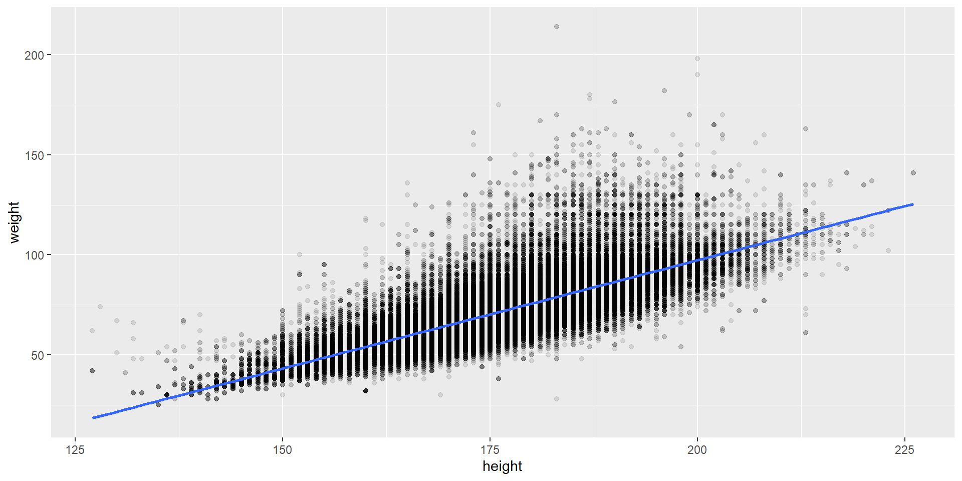
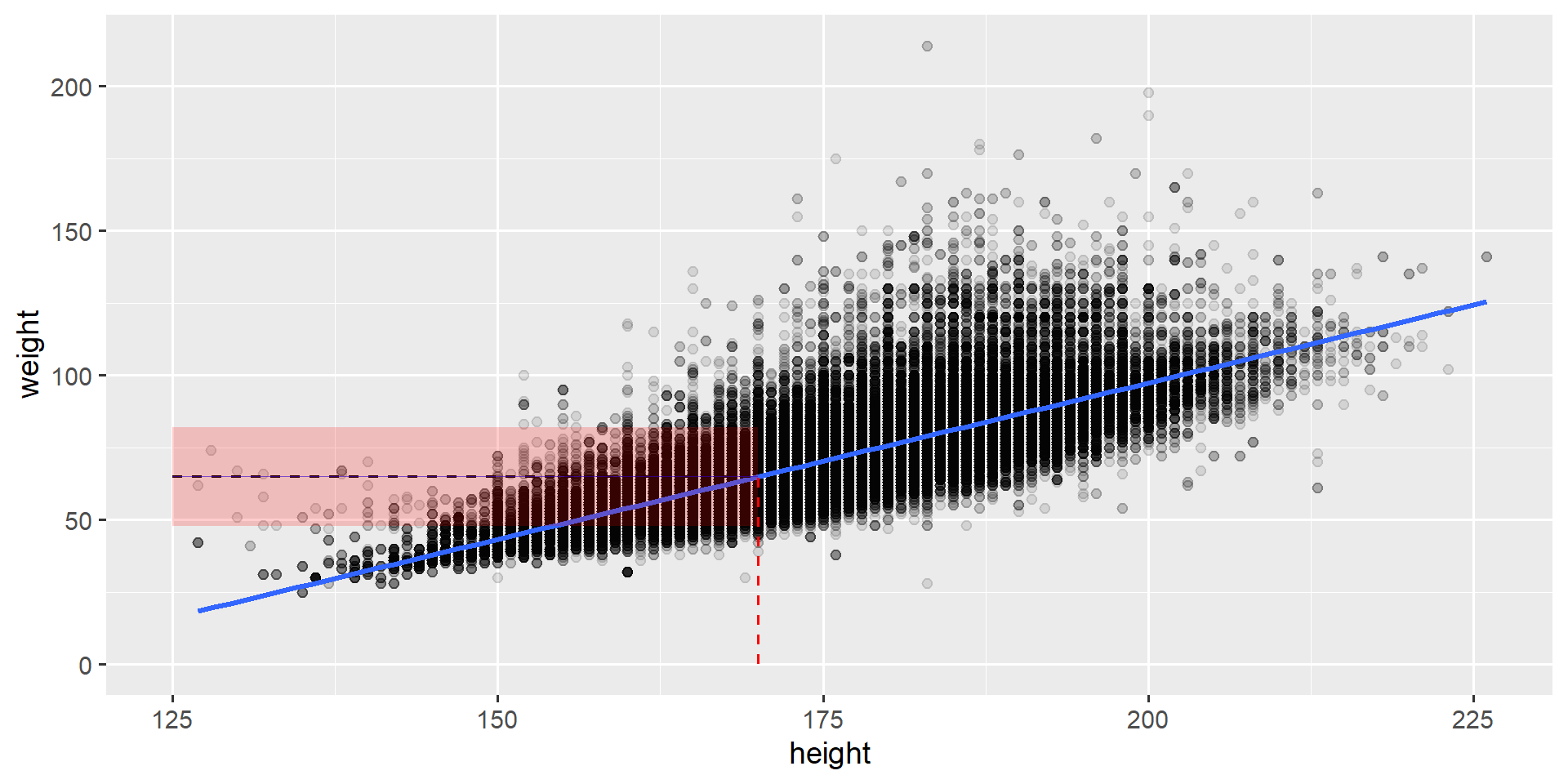
Visualisierung

library(ggplot2)

ggplot(olympics, aes(x = height, y = weight)) +
  geom_point(alpha = 0.1) +
  geom_smooth(method = "lm", se = FALSE)

Lineares Modell

\[weight = \beta_0 + \beta_1 height \]

mod_olympics <- lm(weight ~ height, data = olympics)

broom::glance(mod_olympics)

# A tibble: 1 × 12
  r.squared adj.r.squared sigma statistic p.value    df   logLik      AIC    BIC
      <dbl>         <dbl> <dbl>     <dbl>   <dbl> <dbl>    <dbl>    <dbl>  <dbl>
1     0.634         0.634  8.67   358247.       0     1 -740289. 1480585. 1.48e6
# ℹ 3 more variables: deviance <dbl>, df.residual <int>, nobs <int>

broom::tidy(mod_olympics, conf.int = TRUE)

# A tibble: 2 × 7
  term        estimate std.error statistic p.value conf.low conf.high
  <chr>          <dbl>     <dbl>     <dbl>   <dbl>    <dbl>     <dbl>
1 (Intercept)  -119.     0.318       -375.       0  -120.     -118.  
2 height          1.08   0.00181      599.       0     1.08      1.09

Vorhersagen und Voraussetzungen

Vorhersagen

Wie schwer ist eine Athlet*in mit einer Körpergröße von 170 cm?

new_data <- data.frame(height = 170)
predict(mod_olympics, new_data)

       1 
64.87699 

Confidence Interval: Wie sicher bin ich mir mit dieser Mittelwert-Schätzung?

predict(mod_olympics, new_data, interval = "confidence")

       fit      lwr      upr
1 64.87699 64.83508 64.91891

Prediction Interval: Wie sicher bin ich mir mit der Vorhersage für die eine Person?

predict(mod_olympics, new_data, interval = "prediction")

       fit      lwr      upr
1 64.87699 47.88367 81.87032

Vorhersagen

pred <- predict(mod_olympics, new_data, interval = "prediction")
pred_cft <- predict(mod_olympics, new_data, interval = "confidence")
ggplot(olympics, aes(x = height, y = weight)) +
  geom_point(alpha = 0.1) +
  geom_smooth(method = "lm", se = FALSE) + 
  annotate("segment", x = 125, xend = 170, y = pred[1, "fit"], yend = pred[1, "fit"], color = "black", linetype = "dashed") +
  annotate("rect", xmin = 125, xmax = 170, ymin = pred_cft[1, "lwr"], ymax = pred_cft[1, "upr"], fill = "blue", alpha = 0.6) +
  annotate("rect", xmin = 125, xmax = 170, ymin = pred[1, "lwr"], ymax = pred[1, "upr"], fill = "red", alpha = 0.2) +
  annotate("segment", x = 170, xend = 170, y = 0, yend = pred[1, "fit"], color = "red", linetype = "dashed") +
  theme_grey(base_size = 14)

Voraussetzungen

performance::check_model(mod_olympics, base_size = 7)

Voraussetzungen

• richtige Verteilung, Linearität, Homoskedastizität, keine Ausreißer, Normalverteilung der Residuen, (Multikollinearität)
• Lösungen: anderes Modell, robustes Modell, Transformation der Daten, Ausreißer entfernen